Table of contents
SimilityVectorEmbedding
SimilityVectorEmbedding is a set of Jupyter notebooks that turn a movie catalog into embeddings and look for similar films with several storage and ranking approaches. It is an AlgoÉTS repository for readers who want to see vector search applied to real movie records. The article Exploring movie similarities with vector search algorithms tells the same work as a story, with the original demo animations.
1. Overview
Each folder pairs a notebook with the database it needs. All of them read a movies.json file whose records use French keys (titre, annee, genre, realisateur, role, synopsis …) under films.film.
postgres/0.simple.ipynbis the shortest full path: it builds one text per film (title, year, genres, actors, director, summary, country, language, writers), encodes it withsentence-transformers/all-MiniLM-L6-v2using mean pooling, normalizes the vectors and inserts them into amoviestable with aVECTOR(384)column. Titles typed by the user are matched withpg_trgmbefore cosine similarity ranks the rest of the catalog. It also averages several titles, weights titles by rating, plots the scores and ends with a Gradio interface.postgres/1.create_table.ipynbencodes the same catalog with five configurations (BART, GTE, MiniLM-L12, RoBERTa and e5-large) and stores one vector column per model.postgres/3.LLMS.ipynbembeds a natural-language question, runs a pgvector<=>cosine query and sends the table schema to a LangChain chain backed by Ollama (llama2:13b-chat).qdrant/0.simple.ipynbupserts 384-dimension vectors in batches of 100 into a cosine collection, searches it, and projects the vectors with t-SNE and k-means.bm25/0.bm25.ipynbranks films by keywords withrank_bm25, without embeddings.neo4j/1.create_db.ipynbloads movies and people as a graph and scores neighbours by shared genres, directors, writers and actors.
2. Use cases
Jupyter notebooks that embed a movie catalog and find similar films with pgvector, Qdrant, BM25, Neo4j and Ollama.
- Embed the movie catalog
- LearnerDatabase container
postgres/1.create_table.ipynb builds one text per film from movies.json and encodes it with BART, GTE, MiniLM-L12, RoBERTa and e5-large, storing one vector column per model.
- Find films like a title
- LearnerDatabase container
postgres/0.simple.ipynb resolves the typed title with pg_trgm, then ranks the catalog by cosine similarity for one title, several titles or rated titles.
- Search from a Gradio page
- LearnerDatabase container
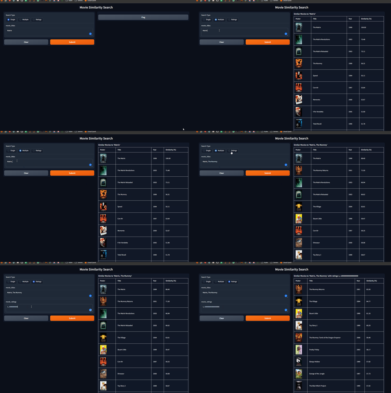
The last cells of postgres/0.simple.ipynb launch a Gradio interface with Single, Multiple and Ratings modes that shows posters, years and similarity scores.
- Search with Qdrant
- LearnerDatabase container
qdrant/0.simple.ipynb upserts 384-dimension MiniLM vectors into a cosine collection, searches it and projects the vectors with t-SNE and k-means.
- Ask a local LLM
- LearnerDatabase containerLocal LLM (Ollama)
postgres/3.LLMS.ipynb embeds a question, runs a pgvector cosine query and passes the schema to a LangChain chain backed by Ollama llama2:13b-chat.
- Compare BM25 and graph search
- LearnerDatabase container
bm25/0.bm25.ipynb ranks films by keywords with rank_bm25, and neo4j/1.create_db.ipynb scores films by shared genres, directors, writers and actors.
2.1. Scenario: Find films like The Matrix
- Start PostgreSQL with pgvector and pg_trgm: cd postgres, then docker-compose up -d.
- Open postgres/0.simple.ipynb with jupyter notebook and run the pip install and import cells.
- Run main() to load movies.json, embed each film with all-MiniLM-L6-v2 and insert it into the movies table.
- Call find_similar_movies(conn, cur, "The Matrix") to get the closest titles above a 0.5 cosine threshold.
- Plot the result with plot_similar_movies or try the same search in the Gradio interface.
Files readREADME.mdpostgres/README.mdpostgres/docker-compose.ymlpostgres/Dockerfilepostgres/init-db.shpostgres/0.simple.ipynbpostgres/1.create_table.ipynbpostgres/3.LLMS.ipynbqdrant/0.simple.ipynbqdrant/docker-compose.ymlbm25/0.bm25.ipynbneo4j/1.create_db.ipynbneo4j/docker-compose.yml
3. How the search works
The PostgreSQL notebooks follow one pipeline. postgres/0.simple.ipynb is the clearest version, so the steps below quote it.
flowchart LR
  J["movies.json<br/>631 films, French keys"] --> P["preprocess_movie_data<br/>flatten roles, director, writers"]
  P --> T["One text per film<br/>title year genres actors director<br/>summary country language writers"]
  T --> E["MiniLM-L6-v2<br/>tokens → masked mean pooling → L2 normalize"]
  E --> DB[("PostgreSQL movies table<br/>embedding_MiniLM VECTOR(384)")]
  Q["Title typed by the user"] --> G["pg_trgm similarity()<br/>best title if score ≥ 0.3"]
  G --> DB
  DB --> V["Query vector<br/>one title, mean of titles,<br/>or rating-weighted mean"]
  V --> C["Cosine similarity<br/>against every other film"]
  C --> R["Keep score > 0.5<br/>sort, top 10"]
  R --> UI["Bar chart or Gradio table"]
3.1. 1. From a JSON record to a text
load_movies_data reads films.film from movies.json; the saved run loads 631 films. preprocess_movie_data maps the French keys to English ones (titre → title, realisateur.__text → director, scenariste → writers) and pulls actor names out of role[].acteur.__text, wrapping a single role in a list first. generate_embedding then glues the fields into one string per film, in this order: title, year, genres, actors, director, summary, country, language, writers. English stopwords are removed from the title and the summary only, with NLTK’s list.
3.2. 2. The embedding
The model is sentence-transformers/all-MiniLM-L6-v2, loaded through Hugging Face AutoModel. The tokenizer truncates each text to 512 tokens and pads the batch. The model returns one 384-dimension vector per token; mean_pooling averages them, multiplying by the attention mask so padding tokens do not count:
token_embeddings = model_output[0]
mask = attention_mask.unsqueeze(-1).expand(token_embeddings.size()).float()
sentence = (token_embeddings * mask).sum(1) / mask.sum(1).clamp(min=1e-9)
F.normalize(..., p=2) then scales every vector to length 1. After that step, cosine similarity and the dot product give the same number.
3.3. 3. The table
setup_database enables the vector, cube and pg_trgm extensions, drops movies if it exists and recreates it with plain columns (title, actors, year, country, language, duration, summary, director, poster), two TEXT[] arrays (genre, scenarists) and embedding_MiniLM VECTOR(384). insert_movie writes each vector as a '[0.01, -0.03, …]' literal, which pgvector parses. No HNSW or IVFFlat index is created, so every search compares the query with every row; for 631 films that is instant.
3.4. 4. Finding the query film
Users type titles loosely, so get_best_matching_title asks pg_trgm for the closest title: ORDER BY similarity(title, %s) DESC LIMIT 1. similarity is the share of three-letter chunks (trigrams) the two strings have in common, from 0 to 1. If the best score is below 0.3 the search stops with “No close match found”. Otherwise the notebook reads that film’s stored vector back.
3.5. 5. Scoring and ranking
find_similar_movies loads every other film’s vector and computes cosine_similarity(query, embeddings) with scikit-learn, in Python. A film is kept when its score is above 0.5, and the top ten are returned in descending order. The two variants only change the query vector:
- Several titles (
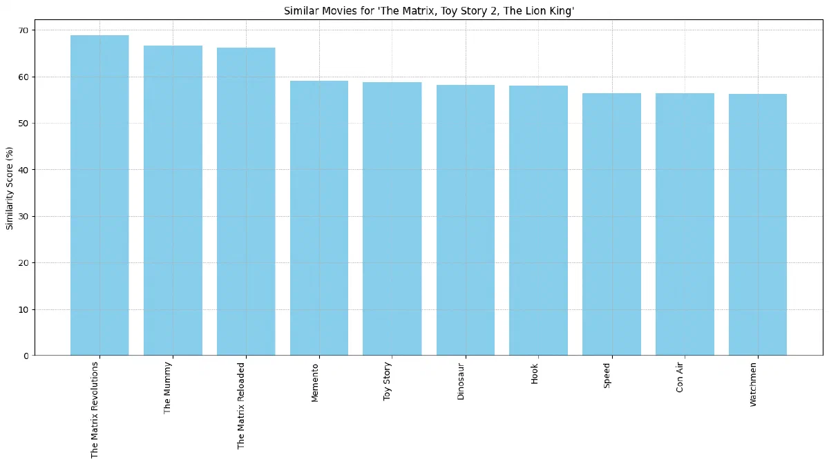
find_similar_movies_list): the plain mean of the titles’ vectors, so a trilogy pulls the search towards what the three films share. - Rated titles (
find_similar_movies_ratings): a weighted mean. The film atinfluential_indexgets weight(rating − 1) × influence_factor; the others keep their rating as weight. With the notebook’s example, The Matrix, Toy Story 2 and The Lion King rated 100, 100 and 1, the weights are 198, 100 and 1, so the query is about two thirds The Matrix, one third Toy Story 2 and almost nothing of The Lion King.
The other notebooks run the same comparison inside the database. 3.LLMS.ipynb orders by 1 - (embedding_MiniLM <=> query): pgvector’s <=> operator returns the cosine distance, so one minus it is the similarity. 2.analyse.ipynb also tries <-> (Euclidean), <#> (negative inner product) and <+> (L1).
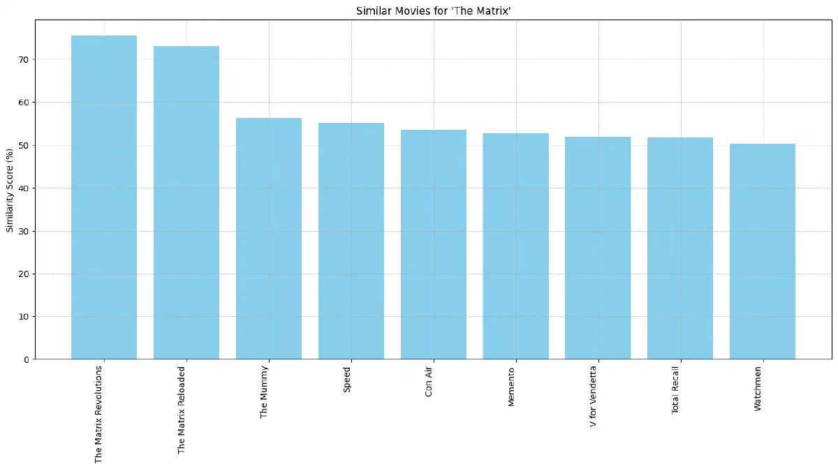
find_similar_movies for The Matrix: the two sequels score about 75% and 73%, then The Mummy, Speed and Con Air in the mid-50s. Nine films pass the 0.5 threshold.
3.6. 6. Choosing a model
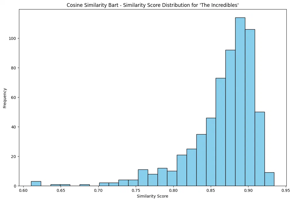
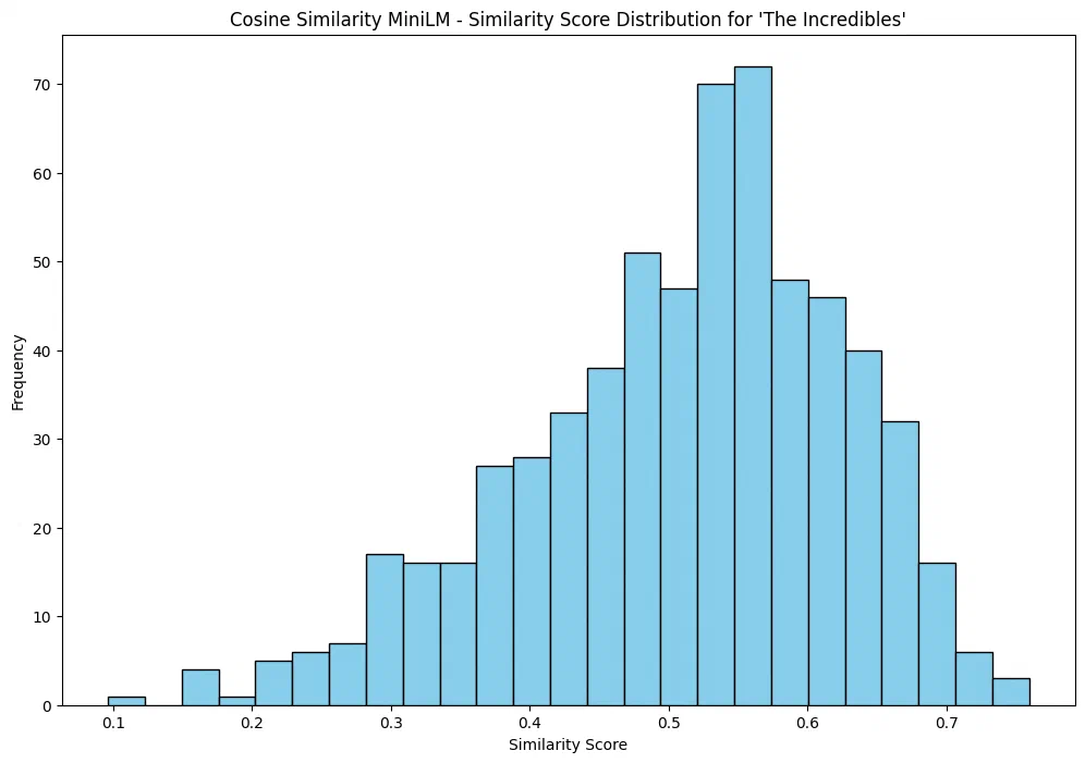
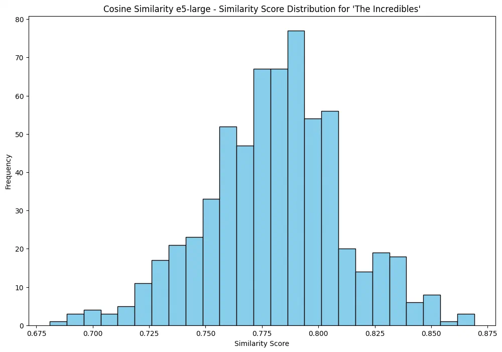
1.create_table.ipynb stores five embeddings per film side by side: facebook/bart-large, Alibaba-NLP/gte-large-en-v1.5 and intfloat/e5-large through AutoModel (1,024 dimensions), and all-MiniLM-L12-v2 (384) and nli-roberta-large (1,024) through SentenceTransformer. 2.analyse.ipynb then plots, for one query film, the cosine score of every other film in the catalog. The spread of those scores matters more than their level: a model whose scores all sit in a narrow band cannot separate a close match from an unrelated film with a fixed threshold.
3.7. 7. Looking at the space
The Qdrant notebook stores the same 384-dimension MiniLM vectors in a cosine collection, then projects them to two dimensions with t-SNE and groups them with k-means. The projection is only a picture: distances in a t-SNE plot are not the cosine scores used for search.
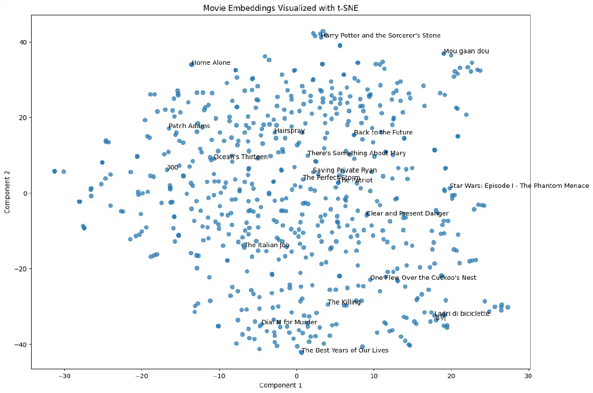
qdrant/0.simple.ipynb.
The Gradio cell wraps the three searches in one page that shows posters, titles, years and scores. This recording comes from the companion article.
4. Getting started
The notebooks install their own packages with !pip install cells. Start the database for the notebook you want to run, then open Jupyter:
git clone https://github.com/AlgoETS/SimilityVectorEmbedding.git
cd SimilityVectorEmbedding/postgres
docker-compose up -d
jupyter notebook
postgres/docker-compose.yml builds PostgreSQL with pgvector compiled from source and pg_trgm, on port 5432. The qdrant/ and neo4j/ folders each have their own docker-compose.yml (Qdrant on 6333/6334, Neo4j on 7474/7687 with APOC and Graph Data Science). neo4j/install_ollama.sh installs Ollama on Linux for the LLM notebook.
5. Repository guide
postgres/0.simple.ipynb: MiniLM embeddings, title matching, single/multiple/rated searches, bar chart and Gradio UI.postgres/1.create_table.ipynb: five embedding models stored side by side in PostgreSQL.postgres/2.analyse.ipynb: score distributions per model and comparisons of cosine, Euclidean, inner-product, Hamming and Jaccard scoring.postgres/3.LLMS.ipynb: question embedding, pgvector query and LangChain + Ollama prompt.postgres/pgvector-archive.ipynb: an earlier all-in-one version of the analysis notebook.postgres/Dockerfile,postgres/docker-compose.yml,postgres/init-db.sh: database image and extension setup.qdrant/0.simple.ipynb,qdrant/docker-compose.yml: the Qdrant version of the search, with clustering plots.bm25/0.bm25.ipynb: keyword ranking baseline.neo4j/1.create_db.ipynb,neo4j/docker-compose.yml,neo4j/personnes.json: graph model of films and people.*/movies.json: the movie catalog, copied into each folder.
6. Features
- build an embedding text from several movie fields, with English stopwords removed from title and summary;
- compare five Hugging Face / Sentence Transformers models on the same catalog;
- store vectors in PostgreSQL with pgvector and match approximate titles with
pg_trgm; - search by one title, the mean of several titles, or a rating-weighted mix of titles;
- run the same idea on Qdrant, then on BM25 keywords and a Neo4j graph for comparison;
- ask questions through a local LLM grounded on the
moviestable; - view results as bar charts, t-SNE/k-means plots, graph views and a Gradio page.
7. Limits
- The README asks for
pip install -r requirements.txtand aSimilarity_Vector_Embedding.ipynbnotebook; neither file is in the repository. Dependencies come from the!pip installcells. - The README schema shows a single
VECTOR(768)column; the notebooks create per-model columns (384 or 1024 dimensions). postgres/init-db.shcreates an extension namedpgvector, while the notebooks createvector, the name pgvector registers.- Notebooks drop and recreate the
moviestable and the Qdrant collection, and use hard-coded local credentials (postgres/postgres,neo4j/password). - The LLM notebook needs a running Ollama server with
llama2:13b-chat; the Gradio cell useslaunch(share=True), which opens a public share link. - In
1.create_table.ipynb, the BART, GTE and e5 vectors arelast_hidden_state.mean(dim=1): the mean includes padding tokens, unlike the masked pooling of the simple notebook, so short summaries are diluted by padding. The e5 model card also asks for apassage:prefix that the notebook does not add. - The search excludes the titles exactly as typed, but looks up the fuzzy-matched title. Typing “the matrix” in lower case can return The Matrix itself as its own best match.
0.simple.ipynbfetches every vector and scores it in Python; only the analysis and LLM notebooks let pgvector do the ranking. No vector index is built.- There are no tests. Saved notebook outputs show past runs, not benchmarks.
8. Sources
- GitHub repository
- README
postgres/0.simple.ipynbpostgres/1.create_table.ipynbpostgres/2.analyse.ipynbpostgres/3.LLMS.ipynb- Companion article: Exploring movie similarities with vector search algorithms
qdrant/0.simple.ipynbneo4j/1.create_db.ipynb
9. CI/CD pipeline
No CI/CD pipeline in the repository. The code is built and run by hand, as described above.
Generated from the source at commit f3db032.
10. Deployment diagram
Mermaid Deployment diagram
flowchart LR
  repo[("GitHub repository")]
  image["Docker image<br/>FROM postgres:latest"]
  subgraph compose["Docker Compose"]
    svc_neo4j["neo4j"]
    svc_pgvector["pgvector"]
    svc_qdrant["qdrant"]
  end
  repo -->|"docker build"| image
  image -->|"docker compose up"| compose
11. External dependencies
The repository declares no external packages: it has no manifest such as pyproject.toml, requirements.txt, package.json or pom.xml.
12. Glossary
Repository
The versioned source files, configuration, and history of a project.
README
The repository’s entry document, usually covering its purpose and initial setup.
Dependency
A library, tool, or service that another component needs to build or run.
HTTP
A request-and-response protocol used by browsers and web services. A method, path, headers, and optional body describe a request.
Container
An isolated process environment created from an image. Persistent data needs storage outside the container’s disposable filesystem.
Docker Compose
A configuration format and tool for starting related containers, networks, and volumes. Startup order alone does not guarantee service readiness.
Volume and bind mount
A volume is storage managed by the container platform; a bind mount exposes a chosen host path inside a container.
Published port
A host port mapped to a service’s container port. Publishing a port can expose that service beyond its container network.
CLI
A text interface in which commands and arguments select operations. Exit codes let scripts detect success or failure.
Build
The steps that turn source files and dependencies into a runnable program or distributable artifact.
Continuous integration
Automated checks that run when source changes, such as building, testing, and linting. Passing checks cover only what those checks exercise.
Mermaid
A text-based diagram language. Nodes and connections describe a model; the diagram itself does not execute the project.
Database
A system for storing and querying structured records. Its schema, access rules, and persistence determine how the application can use that data.
13. References
- AlgoÉTS. (2026, November 5). [Web page] github.com.
- AlgoETS. (2026, November 5). SimilityVectorEmbedding. [Software repository] github.com.
- AlgoETS. (2026, November 5). README. [Source file or documentation] github.com.
- AlgoETS. (2026, November 5). postgres/0.simple.ipynb. [Source file or documentation] github.com.
- AlgoETS. (2026, November 5). postgres/1.create_table.ipynb. [Source file or documentation] github.com.
- AlgoETS. (2026, November 5). postgres/2.analyse.ipynb. [Source file or documentation] github.com.
- AlgoETS. (2026, November 5). postgres/3.LLMS.ipynb. [Source file or documentation] github.com.
- AlgoETS. (2026, November 5). qdrant/0.simple.ipynb. [Source file or documentation] github.com.
- AlgoETS. (2026, November 5). neo4j/1.create_db.ipynb. [Source file or documentation] github.com.
Sources without a publication date show the date they were last checked, November 5, 2026. File links retain the inspected revision where available.