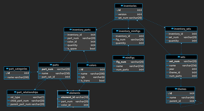
Je collectionne le LEGO et j’écris du Python — croisement des exports Rebrickable avec un scraper BrickEconomy pour voir l’évolution des sets, couleurs et thèmes, et tester une régression simple sur le 001-1. Récit et graphiques ici ; notebooks complets dans AlgoETS/LegosTracker. English version.
Sources
| Source | Apport |
|---|---|
| CSV Rebrickable | sets, thèmes, pièces, couleurs, inventaires |
| BrickEconomy (scrapé) | prix secondaire que Rebrickable ne fournit pas |
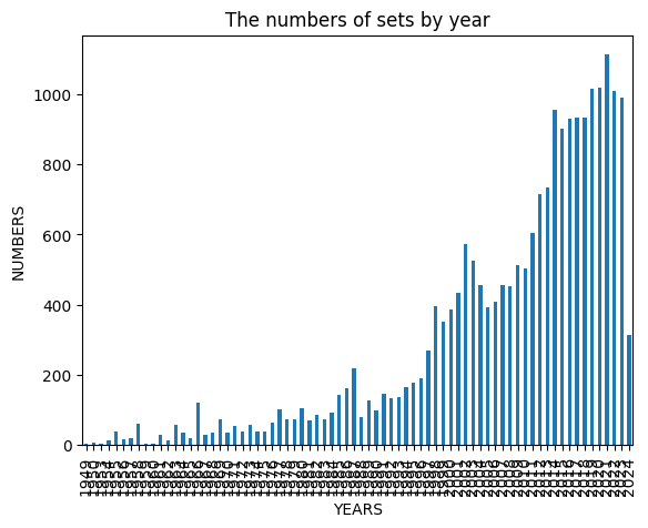
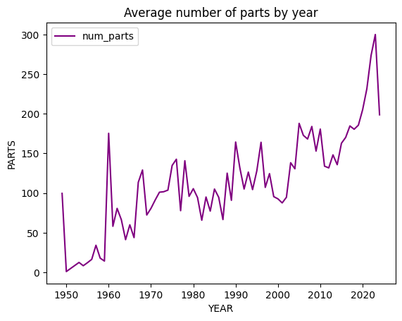
Sets dans le temps
- Nombre de sets par an augmente.
- Pièces moyennes par set monte — modèles plus denses.
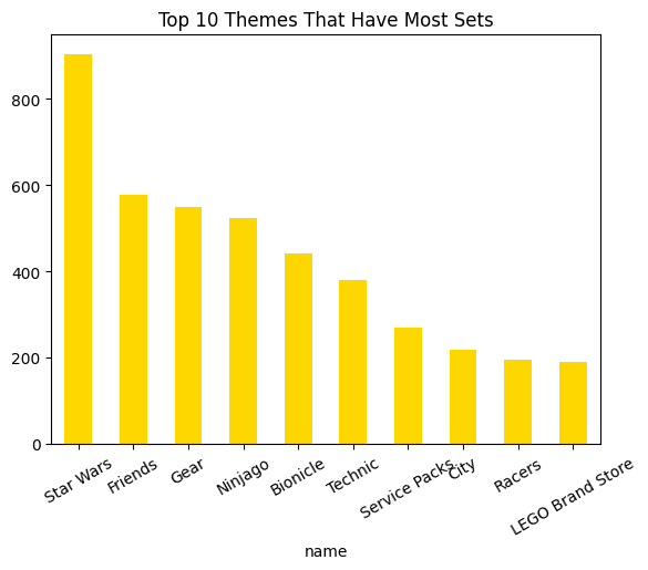
Thèmes dominants
Jointure theme_id, thèmes racine, top 10 par volume.
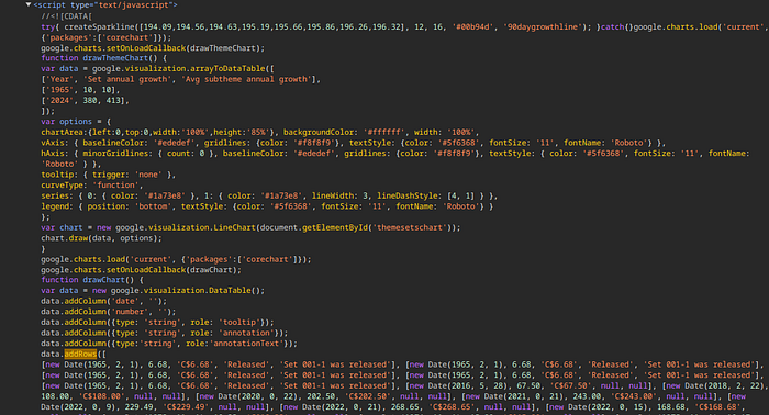
Scraper BrickEconomy
Playwright + asyncio, validation pydantic — code et garde-fous dans le dépôt LegosTracker.
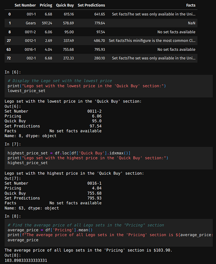
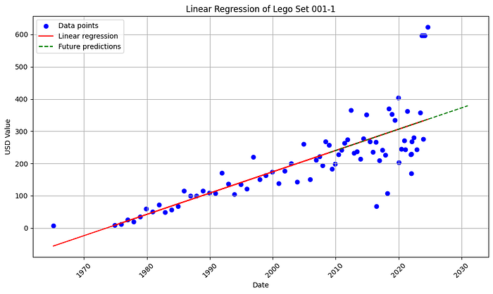
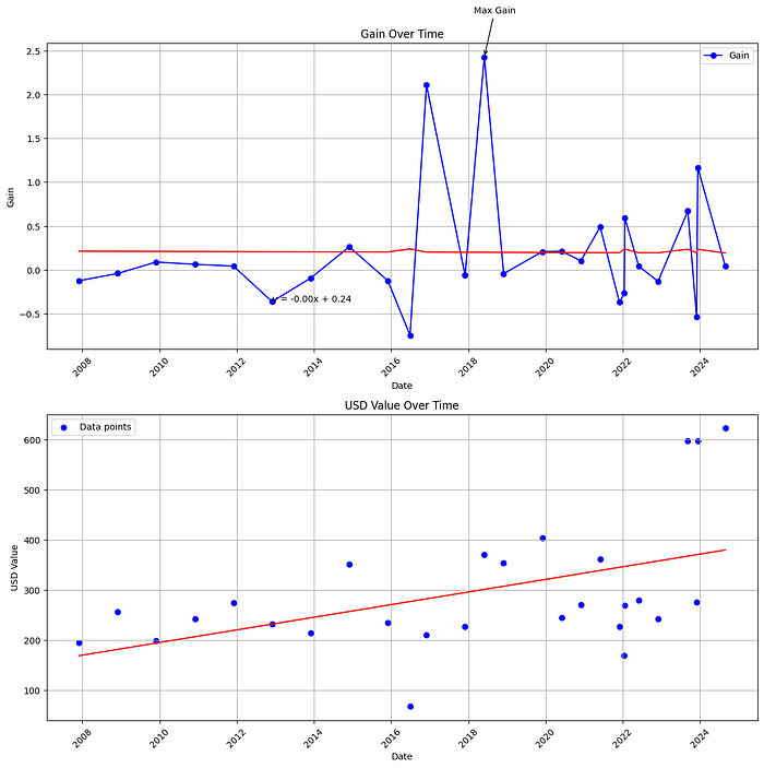
Prix du 001-1
Charger 001-1_history.csv / 001-1_new.csv, nettoyer, tracer dans le temps.
Régression linéaire
Modèle simple pour pratiquer l’interprétation — pas de « alpha » boursier sur la brique.
Détails : Medium et notebooks GitHub.
Extraits notebook
Les one-liners pandas restent dans le dépôt — pas recollés ici.
Limites
Scraper cassé, sets disparus du catalogue, hype collector, confusion MSRP / revente.
Bilan
Données LEGO = pandas + scraping + humilité sur les prix secondaires.
Articles liés
Références
Publié d’abord sur Medium.